Long Short-Term Memory Network for Time Series Forecasting
Long Short-Term Memory Network for Time Series Forecasting
Introduction
To understand the terms frequently used in the context of Machine Learning in a simple way, read my post: Machine Learning Basics.
In practice, basic Recurrent Neural Networks (RNNs) do not seem to be able to learn long-term dependencies. Long Short Term Memory(LSTM) networks are a special kind of RNN, capable of learning long-term dependencies. They were introduced by Hochreiter & Schmidhuber in 1997. LSTMs are explicitly designed to avoid the long-term dependency problem. Remembering information for long periods of time is their default behavior. So LSTM networks are ideal for time series forecasting.
There are many tutorials online that give a theoretical overview of LSTM and its usage. However in this post I will focus on the programmatic implementation of LSTM using Python libraries.
What is Time Series Forecasting?
When we have historical data about anything for example Weather Data or Financial Data or Sales Data or any other data, this data can be used to forecast the future data so that we can have a fair idea of what to expect in the future. This is commonly referred to as Time Series Forecasting or Time Series Prediction.
In this tutorial we will develop a LSTM forecast model for a one-step univariate time series forecasting problem using Python libraries like Keras, scikit-learn, TensorFlow and pandas.
Machine Learning Environment should be setup in your machine. To setup Machine Learning Environment, please refer to my post on: ML Environment Setup.
Here is lstm.py:
Create the LSTM network model using the code:
Requirements to Run the Application
- Anaconda.
- Machine Learning Environment.
- Intellij IDE with Python Community Edition Plugin.
Machine Learning Environment should be setup in your machine. To setup Machine Learning Environment, please refer to my post on: ML Environment Setup.
Step 1: The Dataset
The dataset I have used gives the monthly count of the number of people using public transport in a major city between 2014 and 2016 in Thousands. The dataset is available in GitHub. There are 36 records in the dataset. Please do not use Microsoft Excel to open this file as it does not interpret the Month column correctly. To view or edit this dataset please use a text editor like Notepad or Sublime Text or Notepad++.
Step 2: Create the file: lstm.py
In lstm.py, we will be loading the dataset, building the LSTM network model and perform the time series forecasting using the model.Here is lstm.py:
from pandas import DataFrame
from pandas import Series
from pandas import concat
from pandas import read_csv
from pandas import datetime
from sklearn.metrics import mean_squared_error
from sklearn.preprocessing import MinMaxScaler
from keras.models import Sequential
from keras.layers import Dense
from keras.layers import LSTM
from math import sqrt
from matplotlib import pyplot
import numpy

# Frame the data sequence as a supervised learning problem
def timeseries_to_supervised_learning(data, lag=1):
    df = DataFrame(data)
    columns = [df.shift(i) for i in range(1, lag+1)]
    columns.append(df)
    df = concat(columns, axis=1)
    df.fillna(0, inplace=True)
    return df

# Create a differenced series
def difference_series(dataset, interval=1):
    diff = list()
    for i in range(interval, len(dataset)):
        value = dataset[i] - dataset[i - interval]
        diff.append(value)
    return Series(diff)

#  Function to Parse date-time values for loading the dataset
def parse_dataset(x):
    return datetime.strptime('201'+x, '%Y-%m')

# Inverse the differenced value
def inverse_difference(history, yhat, interval=1):
    return yhat + history[-interval]

# Scale the train and test data to [-1, 1]
def scale_data(train, test):
    # Fit the scaler
    scaler = MinMaxScaler(feature_range=(-1, 1))
    scaler = scaler.fit(train)
    # Transform the train data
    train = train.reshape(train.shape[0], train.shape[1])
    train_scaled = scaler.transform(train)
    # Transform the test data
    test = test.reshape(test.shape[0], test.shape[1])
    test_scaled = scaler.transform(test)
    return scaler, train_scaled, test_scaled

# Invert the scaling for a forecasted value
def invert_scale_value(scaler, X, value):
    new_row = [x for x in X] + [value]
    array = numpy.array(new_row)
    array = array.reshape(1, len(array))
    inverted = scaler.inverse_transform(array)
    return inverted[0, -1]

# Make a one-step forecast
def forecast_lstm(model, batch_size, X):
    X = X.reshape(1, 1, len(X))
    yhat = model.predict(X, batch_size=batch_size)
    return yhat[0,0]

# Fit a LSTM network to the training data
def fit_lstm_network(train, batch_size, nb_epoch, neurons):
    X, y = train[:, 0:-1], train[:, -1]
    X = X.reshape(X.shape[0], 1, X.shape[1])
    model = Sequential()
    model.add(LSTM(neurons, batch_input_shape=(batch_size, X.shape[1], X.shape[2]), stateful=True))
    model.add(Dense(1))
    model.compile(loss='mean_squared_error', optimizer='adam')
    for i in range(nb_epoch):
        model.fit(X, y, epochs=1, batch_size=batch_size, verbose=0, shuffle=False)
        model.reset_states()
    return model

# Load the dataset
series = read_csv('people_count.csv', header=0, parse_dates=[0], index_col=0, squeeze=True, date_parser=parse_dataset)
# Print the first few rows of the input data
print(series.head())
# Plot the dataset
series.plot()
pyplot.show()
# Transform the data to be stationary
raw_values = series.values
difference_values = difference_series(raw_values, 1)

# Transform the data to a supervised learning problem
supervised_learning = timeseries_to_supervised_learning(difference_values, 1)
supervised_values = supervised_learning.values

# Split the data into train dataset and test dataset
train, test = supervised_values[0:-12], supervised_values[-12:]

# Transform the scale of the data
scaler, train_scaled, test_scaled = scale_data(train, test)

# Fit the LSTM model
lstm_model = fit_lstm_network(train_scaled, 1, 200, 3)
# forecast the entire training dataset to build up state for forecasting
train_reshaped = train_scaled[:, 0].reshape(len(train_scaled), 1, 1)
lstm_model.predict(train_reshaped, batch_size=1)

# Rolling Forecast/Walk-forward validation on the test data
predictions = list()
for i in range(len(test_scaled)):
    # Make a one-step forecast
    X, y = test_scaled[i, 0:-1], test_scaled[i, -1]
    yhat = forecast_lstm(lstm_model, 1, X)
    # Invert scaling
    yhat = invert_scale_value(scaler, X, yhat)
    # Invert differencing
    yhat = inverse_difference(raw_values, yhat, len(test_scaled)+1-i)
    # Store the forecast
    predictions.append(yhat)
    expected = raw_values[len(train) + i + 1]
    print('Month:%d, Expected Value:%f, Predicted Value:%f' % (i+1, expected, yhat))

# Report the performance of the LSTM model using RMSE
rmse = sqrt(mean_squared_error(raw_values[-12:], predictions))
print('RMSE: %.3f' % rmse)
# Line plot of observed values vs predicted values
pyplot.plot(raw_values[-12:])
pyplot.plot(predictions)
pyplot.show()
Here is the explanation of the code in lstm.py.
1. Load the dataset from a CSV File using the code:
series = read_csv('people_count.csv', header=0, parse_dates=[0], index_col=0, squeeze=True, date_parser=parse_dataset)
2. Print the first few rows of the input data and plot it in a graph using the code:# Print the first few rows of the input data print(series.head()) # Plot the dataset series.plot() pyplot.show()3. The raw data cannot be used to create a LSTM network model. The data should be transformed. We have 36 records in the input dataset. We will use the first two years of data for the training dataset and the remaining one year of data will be used for the test dataset. Here is the code that has been used for data transformation and for splitting the input dataset into training set and test set:
# Transform the data to be stationary
raw_values = series.values
difference_values = difference_series(raw_values, 1)

# Transform the data to a supervised learning problem
supervised_learning = timeseries_to_supervised_learning(difference_values, 1)
supervised_values = supervised_learning.values

# Split the data into train dataset and test dataset
train, test = supervised_values[0:-12], supervised_values[-12:]

# Transform the scale of the data
scaler, train_scaled, test_scaled = scale_data(train, test)
4. The Batch Size and the Number Of Epochs defines how quickly the LSTM network learns the data. The number of Neurons or Blocks or Number of Memory Units is an important parameter defining a LSTM layer. We will create the LSTM Network Model with a Batch Size of 1, Number of Epochs as 200 and Number of Neurons as 3. These parameters can be tweaked to get better performance from the LSTM Model. The first line of code below specifies these parameters.
Create the LSTM network model using the code:
# Fit the LSTM model
lstm_model = fit_lstm_network(train_scaled, 1, 200, 3)
# forecast the entire training dataset to build up state for forecasting
train_reshaped = train_scaled[:, 0].reshape(len(train_scaled), 1, 1)
lstm_model.predict(train_reshaped, batch_size=1)
5. Now that the LSTM model is trained using the training set, we will evaluate the model on the test data. Here I am using Rolling Forecast or Walk-Forward Model Validation. Each time step of the test dataset will be walked one at a time. THe LSTM network model will be used to make a forecast for the time step, then the actual expected value from the test set will be taken and given to the model for the forecast on the next time step. Here is the code for the same:
# Rolling Forecast/Walk-forward validation on the test data
predictions = list()
for i in range(len(test_scaled)):
    # Make a one-step forecast
    X, y = test_scaled[i, 0:-1], test_scaled[i, -1]
    yhat = forecast_lstm(lstm_model, 1, X)
    # Invert scaling
    yhat = invert_scale_value(scaler, X, yhat)
    # Invert differencing
    yhat = inverse_difference(raw_values, yhat, len(test_scaled)+1-i)
    # Store the forecast
    predictions.append(yhat)
    expected = raw_values[len(train) + i + 1]
    print('Month:%d, Expected Value:%f, Predicted Value:%f' % (i+1, expected, yhat))
6. Report the performance using Root Mean Squared Error(RMSE) and plot a graph of values predicted by the LSTM network model vs the test data or the last one year data in the dataset. Here are a few points to be noted:- The lesser the RMSE the better is the model performance.
- Neural Networks give different results for the same input data as Machine learning algorithms make use of randomness. So different runs of the same program returns different RMSEs.
# Report the performance of the LSTM model using RMSE
rmse = sqrt(mean_squared_error(raw_values[-12:], predictions))
print('RMSE: %.3f' % rmse)
# Line plot of observed values vs predicted values
pyplot.plot(raw_values[-12:])
pyplot.plot(predictions)
pyplot.show()
Step 3: Create file: setup.py
setup.py is used to to build and install the application. Add basic information about the application in setup.py. Once you have this file created, you can build and install the application using the commands:
python setup.py build
python setup.py install
Here is setup.py:
from setuptools import setup

setup(name='LSTM',
      version='1.0.0',
      description='Machine Learning Application to build a LSTM Network Model for TIme Series Forecasting'
      )
python setup.py build python setup.py installHere is setup.py:
from setuptools import setup
setup(name='LSTM',
version='1.0.0',
description='Machine Learning Application to build a LSTM Network Model for TIme Series Forecasting'
)
Run Application:
1. To run the application, in Anaconda Prompt, navigate to your project location and execute the command:
python lstm.py
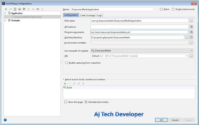
2. To run the application in Intellij IDE, right click the file lstm.py and click Run 'lstm'
Results
1. First a few rows of the input dataset is printed in the logs and then a plot of the input dataset is shown.
 2. A plot of the Test Data i.e. the last year of the input data and the forecast data as evaluated by the LSTM Network Model is displayed.
 3. Here are the complete logs displayed in Intellij. RMSE is 59.399.

1. To run the application, in Anaconda Prompt, navigate to your project location and execute the command:
python lstm.py
2. To run the application in Intellij IDE, right click the file lstm.py and click Run 'lstm'
Results
1. First a few rows of the input dataset is printed in the logs and then a plot of the input dataset is shown.

2. A plot of the Test Data i.e. the last year of the input data and the forecast data as evaluated by the LSTM Network Model is displayed.

3. Here are the complete logs displayed in Intellij. RMSE is 59.399.

Conclusion and GitHub link:
In this post I have shown you how you can create a Long Short-Term Memory Network for Time Series Forecasting using Python libraries. The code used in this post is available on GitHub.
Learn the most popular and trending technologies like Machine Learning, Angular 5, Internet of Things (IoT), Akka HTTP, Play Framework, Dropwizard, Docker, Elastic Stack, Netflix Eureka, Netflix Zuul, Spring Cloud, Spring Boot, Flask and RESTful Web Service integration with MongoDB, Kafka, Redis, Aerospike, MySQL DB in simple steps by reading my most popular blog posts at Software Developer Central.
If you like my post, please feel free to share it using the share button just below this paragraph or next to the heading of the post. You can also tweet with #SoftwareDeveloperCentral on Twitter. To get a notification on my latest posts or to keep the conversation going, you can follow me on Twitter. Please leave a note below if you have any questions or comments.

Comments
Post a Comment